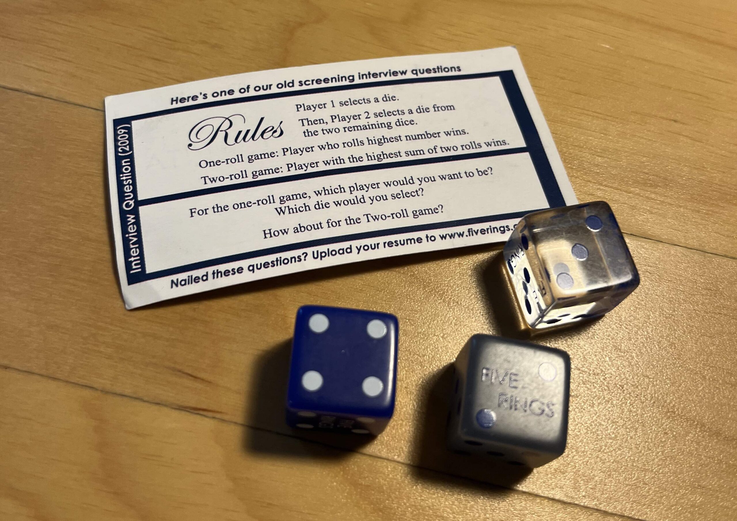
Three-Dice Problem in the Large N Limit

A few years ago, a roommate was going to various career fairs as a rep for his company, and (as one does) he spent some of the time away from his booth collecting swag from other booths. One of the things he picked up was a game (or rather a puzzle) from a quantitative research firm. The image of it is above

You can’t see all the faces of the dice in the photo, so here’s the setup in full.

There are three dice, each of which has six sides. One die has one side with one dot and five sides with four dots. Another die has five sides with three dots and one side with six dots. The last die has three sides with two dots and three sides with five dots. We label the die $D_1$, $D_2$, and $D_3$ respectively.

In this game, Player 1 selects a die. Then Player 2 selects a die from the two remaining dice. In the “one-roll game,” the player who rolls the highest number wins. In the “two-roll game,” the player with the highest sum of two rolls wins.

For the one-roll game, which player would you want to be? Which die would you select?

How about for the two-roll game?

At the time that I found this puzzle, I was re-learning probability and combinatorics in order to develop models of interacting biomolecules. So I thought this question was a good exercise to practice the knowledge I was building. But though the problem setup was simple the results were quite different from what I expected, and naturally led to some extensions:

What would these results be if each die had two arbitrary values $x_{\alpha, 1}$ and $x_{\alpha, 2}$ with respective probability of occurrence $p_{\alpha, 1}$ and $1-p_{\alpha, 1}$ for die $\alpha$?

What would the relative win probabilities be if we rolled each die $N$ times?

What would these results be for $N\gg1$

In this post, we’ll solve the problem as it is stated in Figure 1, but we’ll also consider some of the extensions

Table of Contents

Single-Roll

Naturally, we will consider the single-die roll case first. The hope is that analyzing this simple case could help us develop a structure that can extend to higher-roll cases.

Rock-Paper-Scissors

Say you are playing a game of rock-paper-scissors in which, instead of the two players showing their choices simultaneously, one player goes first and the other player follows. If you wanted to win the game, would you want to be the first player or the second player?

The second player! Given that each choice in the game has another choice that beats it, it would be best to see the other player’s choice first so that you can make the winning selection.

One way to reinterpret the question above is whether this die-roll game is like rock-paper-scissors, and, if so, what is rock, what is paper, and what is scissors?

We have three dice that we label $D_1$, $D_2$, and $D_3$. For each die there is a certain probability of rolling a particular number:
\begin{align}
D_1: &\quad \text{prob $1/6$ of 1 and prob $5/6$ of 4} \\[.5em]
D_2: &\quad \text{prob $5/6$ of 3 and prob $1/6$ of 6} \\[.5em]
D_3: &\quad \text{prob $3/6$ of 2 and prob $3/6$ of 5}.
\end{align}

From the probabilities for each die roll, we can also compute the probabilities of the numbers associated with a pair of dice. Let’s say player 1 chooses $D_1$ and player 2 chooses $D_2$ and they roll a 1 and a 6, respectively. The probability of this combination is the product of the probabilities of obtaining each number: $1/6\times 1/6 = 1/36$. By similar logic, we can compute the probabilities for all four combinations of numbers in a contest between $D_1$ and $D_2$:

\begin{equation}
\text{[$D_1$ vs. $D_2$]} \qquad
\begin{array}{c || c | c }
& 3 & 6 \\ \hline \hline
1 & 5/36 & 1/36 \\[.5em] \hline
4 & \textbf{25/36} & 5/36 \\[.5em]
\label{eq:d1d2}
\end{array}\qquad (1)
\end{equation}

In the far left column of Eq.(1), we list the possible values of a roll of $D_1$. In the top row, we list the possible values of a roll of $D_2$. The elements in the array are the probabilities of a combination in which rolling $D_1$ yields the entry designated by the associated row and rolling $D_2$ yields the entry designated by the associated column.

One player wins when he or she rolls a value that is larger than the other player’s value. In Eq.(1), we wrote in bold the probabilities associated with $D_1$ beating $D_2$. There is only one such probability, so we have

\begin{equation}
\text{$D_1$ beats $D_2$ with probability } \frac{25}{36} = 69.4\%.
\label{eq:d1d2_beats} \qquad (2)
\end{equation}

It is straightforward to create arrays similar to Eq.(1) for the other two possible contests: $D_2$ vs. $D_3$ and $D_3$ vs. $D_1$. For $D_2$ vs. $D_3$ we have the array

\begin{align}
\text{[$D_2$ vs. $D_3$]} \qquad
\begin{array}{c ||c | c }
& 2 & 5 \\ \hline \hline
3 & \textbf{15/36} & 15/36 \\[.5em] \hline
6 & \textbf{3/36} & \boldsymbol{3/36} \\[.5em]
\end{array}
\label{eq:d2d3}\qquad (3)
\end{align}

In Eq.(3), we wrote in bold the probabilities associated with $D_2$ beating $D_3$. Summing these probabilities gives us the total probability that $D_2$ beats $D_3$. Therefore we find

\begin{equation}
\text{$D_2$ beats $D_3$ with probability } \frac{15}{36} + \frac{3}{36} + \frac{3}{36} = \frac{21}{36} = 58.3\%.
\label{eq:d2d3_beats} \qquad (4)
\end{equation}

Similarly, for $D_3$ vs. $D_1$ we have the array

\begin{align}
\text{[$D_3$ vs. $D_1$]} & \qquad
\begin{array}{c ||c | c }
& 1 & 4 \\ \hline \hline
2 & \boldsymbol{3/36} & 15/36 \\[.5em] \hline
5 & \boldsymbol{3/36} & \boldsymbol{15/36} \\[.5em]
\label{eq:d3d1}
\end{array} \qquad (5)
\end{align}

and the probability that $D_3$ beats $D_1$ is

\begin{equation}
\text{$D_3$ beats $D_1$ with probability } \frac{3}{36} + \frac{3}{36} + \frac{15}{36} = \frac{21}{36} = 58.3\%.
\label{eq:d3d1_beats} \qquad (6)
\end{equation}

From Eq.(2), Eq.(4), and Eq.(6), we find that for each die, there is always another die that has a probability greater than $1/2$ (i.e., even odds) of beating it. Therefore, you would always want to be Player 2. More specifically:

(Single-roll game) Answer: You would want to be Player 2 in the single-roll game. If Player 1 chooses $D_1$, you should choose $D_3$, and you would win with $58.3\%$ probability. If Player 1 chooses $D_2$, you should choose $D_1$, and you would win with $69.4\%$ probability. If Player 1 chooses $D_3$, you should choose $D_2$, and you would win with $58.3\%$ probability.

Single-roll game strategy: $D_1$ has one side with one dot and five sides with four dots. $D_2$ has five sides with three dots and one side with six dots. $D_3$ has three sides with two dots and three sides with five dots. For “$x \to y$” in the diagram, $x$ wins against $y$ with the stated probability. We see that for each die, there is another die that wins against it with a greater than $50\%$ chance.

Double-Roll

For the double-roll game, determining which player (either player 1 or 2) we would want to be and which selections we should make requires an analysis similar to that in the single-roll game. The major difference is that for each die, we roll twice and we sum the results of the rolls. For a die that yields the numbers $a$ and $b$ on a single-roll, with probabilities $p_a$ and $p_b$, respectively, the possible summations in a two-roll turn are $2a, a+b$, and $2b$ with probabilities $p_a^2$, $2p_a p_b$, and $p_b^2$, respectively. The probability $2p_a p_b$ comes from the sum of the probabilities of obtaining $a$ then $b$ or $b$ then $a$. For example, the possible sum values for $D_1$ are $2\times 1 = 2$, $1+4 = 5$, and, $2\times 5 =10$ with probabilities $(1/6)^2 = 1/36$, $2(1/6)(5/6) = 10/36$, and $(5/6)^2= 25/36$, respectively. In general, the probability of rolling a particular sum for any of the three dice is

\begin{align}
D_1: &\quad \text{prob $1/36$ of 2, prob $10/36$ of 5, and prob $25/36$ of 8} \\[.5em]
D_2: &\quad \text{prob $25/36$ of 6, prob $10/36$ of 9, and prob $1/36$ of 12} \\[.5em]
D_3: &\quad \text{prob $9/36$ of 4, prob $18/36$ of 7, and prob $9/36$ of 10}
\end{align}

Now, for this two-roll game we can compute the $3\times 3$ arrays analogous to Eq.(1), Eq.(3), and Eq.(5). For $D_1$ vs. $D_2$, we have

\begin{equation}
\text{$D_1$ vs. $D_2$]} \qquad \begin{array}{c ||c | c | c }
& 6 & 9 & 12 \\ \hline \hline
2 & 25/1296 & 10/1296 & 1/1296 \\[.5em] \hline
5 & 250/1296 & 100/1296 & 10/1296 \\[.5em] \hline
8 & 625/1296 & 250/1296 & 25/1296 \\[.5em]
\end{array}
\label{eq:d1d2_2nd} \qquad (7)
\end{equation}

We see that $D_1$ only beats $D_2$ when the former rolls an $8$ and the latter rolls a $6$. This occurs with probability $625/1296$ which is less than $1/2 = 648$. So in $D_1$ vs $D_2$, $D_2$ has a higher likelihood of winning. Given that probabilities must sum to $1$, the probability that $D_2$ beats $D_1$ is

\begin{equation}
\text{$D_2$ beats $D_1$ with probability } 1- \frac{625}{1296} = \frac{671}{1296} = 51.8\% .
\label{eq:d2d1_beats} \qquad (8)
\end{equation}

For $D_2$ vs. $D_3$ we have

\begin{equation}
\text{[$D_2$ vs. $D_3$]} \qquad \begin{array}{c ||c | c | c }
& 4 & 7 & 10 \\ \hline \hline
6 & 225/1296 & 450/1296 & 225/1296 \\[.5em] \hline
9 & 90/1296 & 180/1296 & 90/1296 \\[.5em] \hline
12 & 9/1296 & 18/1296 & 9/1296 \\[.5em]
\end{array}
\label{eq:d2d3_2nd} \qquad (9)
\end{equation}

Computing the probabilities, we find that $D_3$ beats $D_2$ with probability

\begin{equation}
\text{$D_3$ beats $D_2$ with probability } \frac{450}{1296} + \frac{225}{1296} + \frac{90}{1296} = \frac{765}{1296} =59.0\% .
\label{eq:d3d2_beats} \qquad (10)
\end{equation}

Similarly for $D_3$ vs. $D_1$ we have

\begin{equation}
\text{[$D_3$ vs. $D_1$]} \qquad \begin{array}{c ||c | c | c }
& 2 & 5 & 8 \\ \hline \hline
4 & 9/1296 & 90/1296 & 225/1296 \\[.5em] \hline
7 & 18/1296 & 180/1296 & 450/1296 \\[.5em] \hline
10 & 9/1296 & 90/1296 & 225/1296
\end{array}
\label{eq:d3d1_2nd}\qquad (11)
\end{equation}

From which we find that $D_1$ beats $D_3$ with probability

\begin{equation}
\text{$D_1$ beats $D_3$ with probability } \frac{90}{1296} + \frac{225}{1296} + \frac{450}{1296} = \frac{765}{1296} = 59.0\% .
\label{eq:d1d3_beats}\qquad (12)
\end{equation}

So again, from Eq.(8), Eq.(10), and Eq.(12), we find that for whatever die player 1 selects, there is another die that has a greater than $50\%$ chance of beating it. More specifically:

(Double-roll game) Answer: You would want to be Player 2 in the two-roll game. If Player 1 chooses $D_1$, you should choose $D_2$, and you would win with $51.8\%$ probability. If Player 1 chooses $D_2$, you should choose $D_3$, and you would win with $59.0\%$ probability. If Player 1 chooses $D_3$, you should choose $D_1$, and you would win with $59.0\%$ probability.

Double-roll game strategy: For “$x \to y$” in the diagram, $x$ wins against $y$ with the stated probability. We see that for each die, there is another die that wins against it with a greater than $50\%$ chance. We note that the cycle of advantages is reversed relative to that for the Single-roll game.

$N$-Roll

Having considered the incremental cases of single and double-roll games, we will now consider the most general $N$-roll case. From the previous cases, we might guess that the best strategy for the $N$-roll game is to be Player 2. That is, we should wait for the other player to choose a die, then choose the other die with a higher than even chance of beating the die the first player chose. But which die beats which die? The previous cases show that the number of rolls we make can change the cyclic order of wins (e.g., the die that beats another die for a single roll, loses to that other die for the double roll). So we would have to be careful in selecting our chosen die.

Since we are looking for a general result, we won’t write outcome tables like we did before, but will instead find a general expression for the desired probability. First, we put forward some notation. We will label the three dice as $\alpha$, $\beta$, and $\gamma$. The die $\alpha$ can roll the two values $x_{\alpha, 1}$ and $x_{\alpha, 2}$ with probabilities $p_{\alpha, 1}$ and $p_{\alpha, 2} = 1- p_{\alpha, 1}$ respectively.

If we roll the die $\alpha$ $N$ times, the probability that we get $k$ rolls of the value $x_{\alpha, 1}$ and $N-k$ rolls of the value $x_{\alpha, 2}$ is

\begin{equation}
P_{N, \alpha}(k) = \binom{N}{k}\, p_{\alpha, 1}^{k}\, p_{\alpha, 2}^{N-k}. \qquad (13)
\end{equation}

Also, the sum of the values of these $N$ rolls is

\begin{equation}
X_{N, \alpha}(k) = k x_{\alpha, 1} + (N-k) x_{\alpha, 2} \qquad (14)
\end{equation}

The probabilities and dice-rolls sums for the die $\beta$ and $\gamma$ are identical to what is above with the transformation $\alpha \to \beta$ or \(\alpha \to \gamma).

Our goal is to determine the probability that the sum of the dice rolls for die $\alpha$ is greater than the sum of the dice rolls for, say, die $\beta$ when we roll each die $N$ times. We can compute this result by finding the probability for die $\alpha$ to have a sum of values $X_{N, \alpha}$ and for die $\beta$ to have a sum of values of $X_{N, \beta}$ and then summing this probability over all cases where $X_{N, \alpha} > X_{N, \beta}$. The probability for die $\alpha$ to have a particular value of $X_{N, \alpha}(k)$ is P_{N, \alpha}(k). Thus we find that the desired probability is

\begin{equation}
\text{Prob}(X_{\alpha}>X_{\beta}) = \sum_{k=0}^N\sum_{\ell=0}^N P_{N, \alpha}(k)P_{N, \beta}(\ell)\Theta\left(X_{N,\alpha}(k)-X_{N, \beta}(\ell)\right), \qquad (15)
\end{equation}

where we defined the Heaviside step function $\Theta$ as

\begin{equation}
\Theta(x) \equiv \begin{cases} 1 & x>0 \\[.5em] 0 & \text{otherwise} \end{cases}. \qquad (16)
\end{equation}

or written more expansively

\begin{align}
\text{Prob}(X_{\alpha}>X_{\beta}) &= \sum_{k=0}^N\sum_{\ell=0}^N \binom{N}{k} \binom{N}{\ell} p_{\alpha, 1}^{k}\, p_{\alpha, 2}^{N-k}\, p_{\beta, 1}^{\ell}\, p_{\beta, 2}^{N-\ell} \\
& \qquad \qquad \times \Theta\left(k x_{\alpha, 1} + (N-k) x_{\alpha, 2}-\ell x_{\beta, 1} -(N-\ell) x_{\beta, 2}\right). \qquad (17)
\label{eq:prob_alpha_beta}
\end{align}

Eq.(17) is the desired general result. It gives us the probability that any die $\alpha$ beats any other die $\beta$, and we can use it to affirm the results of the previous sections for $N=1$ and $N=2$. But for larger $N$, the calculation would benefit from some numerical packages.

Theory and Simulations

To get a sense for how the win probability for say die $alpha$ over die $beta$ varies with $N$ we could plot Eq.(17) as a function of $N$. Alternatively, we could simulate the die-rolling game multiple times and count the number of times one die beats the other. We will do both.

First, we define arrays for the probabilities and the values of each die:

import numpy as np
# parameter definitions

# vector of values
x = np.array([[4, 1],
              [6, 3],
              [5, 2]])

# vector of probabilities
p = np.array([[5/6,1/6],
                     [1/6,5/6],
                     [1/2,1/2]])

Next, we write Eq.(17) using numpy and scipy libraries:

from scipy.special import comb

# defining probability difference function
prob_diff = lambda alpha, beta, N: np.sum([[comb(N, k, exact=True)*p[alpha][0]**(k)*p[alpha][1]**(N-k)
                                            *comb(N, l, exact=True)*p[beta][0]**(l)*p[beta][1]**(N-l)
                                            *np.heaviside(k*(x[alpha,0]-x[alpha,1])-l*(x[beta,0]-x[beta,1]) 
                                                          - N*(x[beta,1]-x[alpha,1]),0) 
                                            for k in range(N+1)] 
                                           for l in range(N+1)])

With this function, plotting Eq.(17) is then easy.

For the simulation, we use numpy.random to simulate the binomial draws of rolling a die multiple times. Selecting only those draws for which one die beats the other, we can then calculate a win percentage by dividing the total number of wins by the number of runs of the simulation:

def dice_simulator(alpha, beta, N, Nsim=10000, p = p, x = x):
    
    # empty list counting wins
    win_list = list()

    # running simulation 
    for k in range(Nsim):
        
        # rolling the two dice N times
        k_alpha = np.random.binomial(N, p[alpha_,0])
        k_beta = np.random.binomial(N, p[beta_,0])

        # tallying totals
        X_alpha = k_alpha*x[alpha_,0] + (N-k_alpha)*x[alpha_,1]
        X_beta = k_beta*x[beta_,0] + (N-k_beta)*x[beta_,1]

        # adding 1 if alpha beats beta
        if X_alpha > X_beta:
            win_list.append(1)
        else:
            win_list.append(0)    
    
    # gives probability that dice alpha beats dice beta
    return np.sum(win_list)/Nsim

With these two functions, we can now plot both the exact theoretical results and the simulation results for die 1 competing with die 2.

(Figure 2 : Theory and Simulation plots for $N$ roll game. We see that $D_1$ doesn’t always beat $D_2$ and instead the win probability oscillates roughly about 0.5 as $N$ increases.)

From the figure, we see that the probability that $D_1$ beats $D_2$ oscillates about the $0.5$ line with every third value being approximately $0.5$, and the values on either side of it being more significantly above or below this halfway point.

Thus for $1, 4, 7, \ldots$ rolls, $D_1$ has a significant chance of beating $D_2$, but this chance decreases for increasing number of rolls. Alternatively, for $3, 6, 9, \ldots$ rolls $D_2$ has a significant chance of beating $D_1$, and this chance also decreases with $N$. For $2, 5, 8, \ldots$ rolls, there is a slightly more than half chance that $D_2$ beats $D_1$, but this incremental chance again decreases for increasing $N$. We can show that the pairs $D_2$ and $D_3$ and $D_3$ and $D_1$ have similar relationships.

Thus, we have a strategy for the general $N$ roll game: For $N\, \text{mod}\, 3 =1$, $D_1$ beats $D_2$. Otherwise $D_2$ beats $D_1$, doing so slightly if $N\, \text{mod}\, 3 =2$ and more signficiantly if $N\, \text{mod}\, 3 =0$. The same ordering applies if we change $D_1 \to D_2$ and $D_2 \to D_3$ or $D_1 \to D_3$ and $D_2 \to D_1$.

($N$-roll game) Answer: You would want to be Player 2 in any $N$ roll game. If Player 1 chooses $D_1$, you should choose $D_3$ if $N\, \text{mod}\, 3 =1$. Otherwise, you should choose $D_2$. If Player 1 chooses $D_2$, you should choose $D_1$ if $N \, \text{mod}\, 3 =1$, otherwise you should choose $D_3$. If Player 1 chooses $D_3$, you should choose $D_2$ if $N \, \text{mod}\, 3 =1$, otherwise you should choose $D_1$.

Large $N$ Limit

So, we’ve solved the first two additional problems in the above extensions to the original problem. Namely, we found a general expression for the win probability of one die over another for arbitrary probability and face values. And we also found how this expression changes as we increase $N$. Now we will approach the final task of considering these results in the $N\gg 1$ limit.

This final task should be simple given the statistical tools at our disposal, but we will find that the simple path leads to too simple of an answer, thus requiring us to delve into some additional methods to find a different perspective.

Central Limit Theorem

The reason this should be simple is that we are dealing with distributions which have well-defined means and variances, and therefore, by the central limit theorem, assume a common form in the large $N$ limit.

For die $\alpha$, the theoretical average value of $N$ rolls is

\begin{equation}
\mu(N, \alpha) = N x_{\alpha, 1} p_{\alpha, 1} + N x_{\alpha, 2} p_{\alpha, 2}. \qquad (18)
\end{equation}

and the theoretical variance in the value of these $N$ rolls is

\begin{align}
\sigma^2(N, \alpha) & = N(x_{\alpha, 1}^2 p_{\alpha, 1} + x_{\alpha, 2}^2 p_{\alpha, 2})- N(x_{\alpha, 1} p_{\alpha, 1} + x_{\alpha, 2} p_{\alpha, 2})^2\\
& = N(x_{\alpha, 1}- x_{\alpha, 2})^2 p_{\alpha, 1} p_{\alpha, 2}. \qquad (19)
\end{align}

Therefore, by the central limit theorem, the probability distribution for the sum of $N$ rolls of die $\alpha$ has the large $N$ form

\begin{equation}
P_{N}(X_{\alpha}) \stackrel{N\gg1}{\longrightarrow} \frac{1}{\sqrt{2\pi \sigma^2(N, \alpha)}} \exp\left[ -\frac{1}{2\sigma^2(N, \alpha)}\left(X_{\alpha}\, – \mu(N, \alpha)\right)^2\right]. \qquad (20)
\end{equation}

We could have also derived this result directly by expanding Eq. (13) in the $N\gg1 $ limit. With Eq. (20), we can ask what is the probability that $X_{\alpha}> X_{\beta}$ for $N$ rolls. To answer this, we will first find the probability distribution of the difference $U_{\alpha -\beta} = X_{\alpha}- X_{\beta}$. By the convolution properties of the Gaussian, we know that the distribution $U_{\alpha -\beta}$ has mean $\mu(N, \alpha)-\mu(N, \beta)$ and variance $\sigma^2(N, \alpha) + \sigma^2(N, \beta)$. The probability distribution is therefore

\begin{equation}
P_{N}(U_{\alpha-\beta}) \simeq \frac{1}{\sqrt{2\pi (\sigma^2(N, \alpha) + \sigma^2(N, \beta))}} \exp\left[ -\frac{1}{2\sigma^2(N, \alpha)}\left(X_{\alpha}\, – \mu(N, \alpha)+\mu(N, \beta)\right)^2\right].\qquad (21)
\end{equation}

We can in turn approximate the probability that $X_{\alpha}> X_{\beta}$ as

\begin{equation}
\text{Prob}(X_{\alpha}>X_{\beta}) \simeq \int^{\infty}_{0} dU_{\alpha-\beta}\,P_{N}(U_{\alpha-\beta}), \qquad (22)
\end{equation}

which yields

\begin{equation}
\text{Prob}(X_{\alpha}>X_{\beta}) \simeq \frac{1}{2} \left[1+ \text{erf}\left(\frac{\mu(N, \alpha)-\mu(N, \beta)}{\sqrt{2(\sigma^2(N, \alpha) + \sigma^2(N, \beta))}}\right)\right]. \qquad (23)
\label{eq:probNlarge}
\end{equation}

This answer seems clean enough. However, if we were to calculate $\mu(N, \alpha)$ for all of our dice, we would find they all have the same expected value. Therefore, Eq.(23) would predict that there is a 50-50 chance any die beats any other in the $N\gg1$ limit.

However, we know this is not true given the plot Figure 2. In the plot, there are indeed points that seem to approximate $0.5$ as $N$ increases, but there also seems to be a profile of points that remain just above and below 0.5 to not be negligible. Somehow our central limit approximation of the probability distribution is yielding too approximate of a result and is washing away some necessary variance.

Method of Steepest Descent

The central limit theorem gave us an answer, but that answer was too simple. So let’s try something a bit less formulaic (but only a bit!). We return to Eq.(17). One way to implement a large $N$ limit is to transition the discrete sums or combinatorial factors into a continuous space for which such approximations are easy. That is essentially what we were doing to the binomial factors $\binom{N}{k}$ when we implemented the central limit theorem. But it is also possible to do with the Heaviside step function. Given the contour integral definition of the Kronecker delta, we find that we can write the step function as

\begin{equation}
\Theta(M) = \sum_{k=1}^{\infty}\delta(M, k)= \frac{1}{2 \pi i} \oint_{\Gamma} \frac{dz}{z^{M+1}}\sum_{k=1}^{\infty} z^k = \frac{1}{2 \pi i} \oint_{\overline{\Gamma}}\frac{dz}{z^{M+1}}\frac{z}{1-z}, \qquad(24)
\end{equation}

where $\Gamma$ is a closed contour around the origin in the complex plane, and $\overline{\Gamma}$ is a closed contour for which $|z|$ is always less than 1. With this form for the step function, we can rewrite Eq.(17) in terms of a contour integral and then perform the summations over $k$ and $\ell$ to obtain an expression written only as an integration. Doing so, we find

\begin{equation}
\text{Prob}(X_{\alpha}>X_{\beta}) = \frac{1}{2\pi i } \oint_{\overline{\Gamma}} \frac{dz}{1-z}\big(p_{\alpha, 1} z^{-x_{\alpha, 1}} + p_{\alpha, 2} z^{-x_{\alpha, 2}}\big)^N\big(p_{\beta, 1} z^{x_{\beta, 1}} + p_{\beta, 2} z^{x_{\beta, 2}}\big)^N. \qquad (25)
\end{equation}

To prepare for the steepest descent approximation, we write the above expression in the alternative form

\begin{equation}
\text{Prob}(X_{\alpha}>X_{\beta}) = \frac{1}{2\pi i } \oint_{\overline{\Gamma}} dz\, \exp F_{N}(z; \hat{p}; \hat{x}), \qquad (26)
\end{equation}

where we defined

\begin{equation}
F_{N}(z; \hat{p}, \hat{x}) \equiv -\ln\left(1-z\right) + N \ln\big(p_{\alpha, 1} z^{-x_{\alpha, 1}} + p_{\alpha, 2} z^{-x_{\alpha, 2}}\big)+N \ln\big(p_{\beta, 1} z^{x_{\beta, 1}} + p_{\beta, 2} z^{x_{\beta, 2}}\big), \qquad (27)
\end{equation}

where $\hat{p}$ is the matrix of probabilities for the two dice, and $\hat{x}$ is the matrix of values for the two dice. With the desired probability expressed as an integral in Eq.(26), we can in turn apply the method of steepest descent to approximate the result. The approximation yields the expression

\begin{equation}
\text{Prob}(X_{\alpha}>X_{\beta}) = \frac{1}{\sqrt{2\pi \,\partial_z^2F_{N}(z_0; \hat{p}, \hat{x})}}\exp F_{N}(z; \hat{p}; \hat{x}), \qquad (28)
\end{equation}

where $z_0$ is defined by $\partial_{z} F_{N}(z; \hat{p}; \hat{x})|_{z=z_0} = 0 $¹. We cannot compute an analytical solution to the critical point condition that defines $z_0$, but we can compute the value numerically. Doing so and inserting the found value into Eq.(28) yields an approximate expression for this probability as a function of $N$.

We can plot the result of this procedure in the same plot where we depicted the simulation and exact theoretical results.

(Figure 3 : Theory, Simulation, and Large $N$ plots for $N$ roll game. The “Large $N$” plot appears to reproduce only the $N\gg1$ behavior of the minimum of the probability profile.)

In Figure 3, we denote the points arising from Eq.(28) as green circles. We see that asymptotically this large $N$ limit reproduces only the minimum of the probability profile of the exact result. So although the method of steepest descent approach to the large $N$ properties of this game gives us something better than the 0.5 steepest descent result, it still doesn’t yield a result with the oscillatory properties of the exact solution².

Final Remarks

OK! So that was quite the journey. We started with an apparently simple dice roll game and ultimately ventured into combinatorics, simulations, the central limit theorem, and complex analysis. The initial simplicity of the game hid a lot of structure which we only further explored by asking some questions that naturally followed from the original prompt. We did leave some questions on the table though, two particularly important ones for better understanding this game and others like it have to do with the two odd properties we found:

Cyclic Wins: What determines the cyclic properties between the three dice? Can we find a general condition on the values and probabilities for which three dice satisfy this “rock-paper-scissors” relationship for their win probabilities?
Periodic Probabilities: What determines the period of oscillations for the probability that one die beats another? Can such a period be written in terms of the probabilities and values of each die roll?

Answering these questions would have to wait for another time.

Companion Notebook

https://github.com/mowillia/abstractions/blob/main/2023_24_09_n_dice_problem.ipynb

We are skipping over in deriving Eq.(28), in particular details concerning the disappearance of the factor of $1/i$. A standard complex analysis reference (like the Complex Analysis chapter of Hassani, S. (2013). Mathematical physics: a modern introduction to its foundations. Springer Science & Business Media) would provide a formal treatment of the method of steepest descent. ↩︎
However, something tells me that a contour integral approach should be able to reproduce the observed oscillatory behavior for the fairly naive fact that contour integral involves complex numbers which can be expressed in terms of complex exponentials which themselves are typically associated with oscillatory dynamics in modeling. ↩︎