Can we compute the velocity-scaling behavior of drag forces using the simple model of an object moving through a gas cloud?
When physicists discuss the “drag force” experienced by an object due to its interaction with an ambient environment, they typically specify the drag force as one proportional to \(v\) or one proportional to \(v^2\). The former is termed laminar (or Stokes) drag and is experienced by objects moving at low Reynolds number (typically corresponding to low velocity). The latter is termed turbulent drag and is experienced by objects moving at high Reynolds number (typically corresponding to high velocity). Deriving the exact expression for these drag forces requires some results from fluid dynamics, but one can qualitatively reproduce the results of various velocity-dependent regimes of the drag force using a simple many-particle collision system.
Introduction
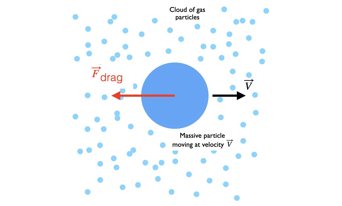
Say that a massive point particle moves in a straight line through a uniform cloud of much smaller particles. Because the massive point particle is moving in a single dimension, it effectively experiences a constant linear mass density $\lambda$ from the cloud of particles. Say also that the cloud of particles is motile and has a velocity probability distribution given by $p(v)$. Given this setup, our objective is to compute the collective force experienced by the massive particle from the cloud. This collective force is the “drag force” experienced by the massive particle.

(Figure 1: Massive particle moving with velocity \(\vec{V}\) through a cloud of particles experiences a drag force opposing its motion. How does this drag force depend on the velocity distribution of the cloud of particles?)
Drag Force Integral
We want to compute the drag force on the massive particle from its collisions with the cloud of particles. Since the cloud of particles has a velocity distribution given by \(p(v)\), we can expect this drag force to be expressed as some integral over this distribution.
As a general outline of our calculation, we will first compute the force a particle experiences from a collision with an infinitesimally small particle (labeled as ISP to distinguish it from the particle), hitting it from the front or hitting it from behind. We will then compute the expectation value of this force using our conjectured probability distribution for velocity, \(p(v)\). This will give us the average force felt by the particle along its trajectory. For simplicity, we will assume that the ISPs collide elastically with the particle.

(Figure 2: Collisions with front and back of massive particle. In the “Lab Frame,” both particles are moving. In the “Fixed Target” frame, the massive particle (i.e., the target) is fixed in place.)
First considering the particle colliding with a single ISP, we have the situations depicted in Figure 2. On the left side of the figure, an ISP of mass \(m\) travels in front of the particle. The ISP is moving with a velocity of \(V-v\) relative to the particle where \(V\) is the particle velocity and \(v\) is the ISP velocity. We note that the ISP will only collide with the particle if the ISP’s velocity is less than the particle’s velocity, that is if \(v-V<0\). If we assume the mass of the particle is much larger than the mass of the ISP, then in the rest frame of the particle the ISP is reflected straight in the opposite direction with the same magnitude of velocity.
Given the domain of allowed values of \(v\) we can then state that the impulse imparted to the particle from a front-end collision with an ISP is
\begin{equation}
\Delta p_{\text{front}} = -2m(V-v) \qquad \text{for \(v \in (-\infty,+V)\)}. \qquad (1)
\end{equation}
Similarly, the impulse imparted to the particle from a back-end collision with an ISP is
\begin{equation}
\Delta p_{\text{back}} = +2m(v-V) \qquad \text{for \(v \in (+V,\infty)\)}. \qquad (2)
\end{equation}
Now, given that the spatial density of ISPs is uniform, we can define a constant linear mass density $\lambda$ along the particle’s trajectory. Also since we assume the particle moves in a straight line, the linear density of ISPs will result in the particle experiencing a series of impulse changes over time. These impulse changes add up to the force the ISP experiences.
Generally, if the collisions are occurring every \(\Delta t\) seconds and inducing a momentum change change of \(\Delta p \), then the force, exerted on the particle is
\begin{equation}
F = \frac{\Delta p}{\Delta t} = \frac{\Delta p}{\Delta x} \frac{\Delta x}{\Delta t}, \qquad (3)
\end{equation}
where $\Delta x$ is the distance between the two impulse changes. For our system, $m/\Delta x \equiv \lambda$, and $\Delta x/\Delta t$ is the relative velocity between the particle and the ISP. Therefore, given Eq.(1) and Eq.(2), we find that the forces for the front and back end collisions are
\begin{align}
F_{\text{front}} &= -2\lambda(V-v)^2 \qquad \text{for \(v \in (-\infty,+V)\)},\\
F_{\text{back}} &= +2\lambda(v-V)^2 \qquad \text{for \(v \in (+V,\infty)\)}.
\end{align}
Finally, for a probability density which is valid for the entire real domain of velocity values, we can compute the expectation value of the external force on the particle as a function of the particle velocity \(V\). We have
\begin{equation}
\langle F_{\text{ext.}}(V) \rangle = 2\lambda \left[-\int^{V}_{-\infty}dv\, p(v) (V-v)^2+ \int_{V}^{\infty}dv\, p(v) (V-v)^2\right] \qquad (4)
\end{equation}
We term Eq.(4) the “drag force integral,” and it generally applies to any probabilistic velocity distribution of constant-density ISPs. Next, we will choose a physically motivated probability density to derive some more precise results for the average force.
Boltzmann Distribution
For a cloud of particles in a room, the standard probability distribution for their velocities is known as the Maxwell-Boltzmann distribution. This distribution has the general form of a Gaussian, so that we may write
\begin{equation}
p(v) = \frac{1}{\sqrt{2\pi \sigma^2}} e^{-v^2/2\sigma^2}.\qquad (5)
\label{eq:pv}
\end{equation}
where \(\sigma^2 = k_BT/m\) for ISPs with mass \(m\), Boltzmann constant \(k_B\), and system temperature \(T\). Note, that we want the probability distribution of velocity in one dimension and not the probability distribution of speed which comes with an additional quadratic factor of \(v\).
Inserting Eq.(5) into Eq.(4) and using some integration identities, we find
\begin{align}
\langle F_{\text{ext.}}(V)\rangle & = \frac{2\lambda}{\sqrt{2\pi\sigma^2}} \left[-\int^{V}_{-\infty} dv\, e^{-v^2/2\sigma^2}(V-v)^2 +\int^{\infty}_{V} dv\, e^{-v^2/2\sigma^2}(v-V)^2 \right] \\
& = \frac{\lambda}{\sigma}\sqrt{\frac{2}{\pi}}\left[-\int^{-V}_{-\infty} dv\, e^{-v^2/2\sigma^2}(V-v)^2 -\int^{V}_{-V} dv\, e^{-v^2/2\sigma^2}(V-v)^2 \right.\\
& \hspace{4cm} \left.+\int^{\infty}_{V} dv\, e^{-v^2/2\sigma^2}(v-V)^2 \right] \\
& = \frac{\lambda}{\sigma}\sqrt{\frac{2}{\pi}}\left[\int^{\infty}_{V} dv\, e^{-v^2/2\sigma^2}\left[(v-V)^2-(V+v)^2\right] -\int^{V}_{-V} dv\, e^{-v^2/2\sigma^2}(V-v)^2 \right],
\end{align}
and thus we have
\begin{equation}
\langle F_{\text{ext.}}(V)\rangle = -\frac{\lambda}{\sigma}\sqrt{\frac{2}{\pi}}\left[4V \sigma^2e^{-V^2/2\sigma^2}+\int^{V}_{-V} dv\, e^{- v^2/2\sigma^2}(V-v)^2 \right]. \qquad (6)
\end{equation}
Eq.(6) is an integral so from it alone, it is difficult to get an intuitive sense of the functional form we expect for the force. So as a next step, we consider some limiting cases for this expression. These cases will be analogous to the ones we consider in a fluid-dynamic model of the “gas” of particles.
Low-Velocity Limit
We consider Eq.(6) in the \(V \ll \sigma \) limit. This corresponds to the velocity of the particle being much lower than the RMS velocity of the ISPs in the cloud1. In this limit the Gaussian factors \(e^{-V^2/\sigma^2}\) and \(e^{-v^2/\sigma^2}\) both approximate to 1 (the latter approximation obtained by considering the domain of integration). We thus find
\begin{align}
\langle F_{\text{ext.}}(V)\rangle & \simeq -\frac{\lambda}{\sigma}\sqrt{\frac{2}{\pi}}\left[4V \sigma^2 + \int^{V}_{-V} dv \, (V-v)^2\right]\\
& = – 4\lambda \sigma \sqrt{\frac{2}{\pi}} V \qquad (7)
\end{align}
Thus we find in this low-velocity limit, the drag force goes as \(\langle F_{\text{ext.}}\rangle \sim V\) and is thus linear in \(V\).
High-Velocity Limit
With the approximation \(V \gg \sigma\) we can replace gaussians with Dirac delta functions as established by the limit
\begin{equation}
\lim_{\sigma \to 0} \frac{1}{\sqrt{2\pi \sigma^2}} e^{-v^2/\sigma^2} = \delta(v).
\end{equation}
Doing so in Eq.(6) gives us
\begin{align}
\langle F_{\text{ext.}}(V)\rangle & \simeq -\frac{\lambda}{\sigma}\sqrt{\frac{2}{\pi}}\left[4V \sigma^3 \sqrt{2\pi}\delta(V) +\sqrt{2\pi}\sigma \int^{V}_{-V} dv \,\delta(v) (V-v)^2\right]\\
& = -2 \lambda V^2, \qquad (8)
\end{align}
where we dropped the first term because of the \(V\gg \sigma>0\) assumption. Thus we find in this high-velocity limit, the drag force goes as \(\langle F_{\text{ext.}}\rangle \sim V^2\) and is thus quadratic in \(V\).

(Figure 3: For a massive particle moving in a cloud of smaller particles with gaussian distributed velocities, the force felt on the massive particle is linear or quadratic depending on how its velocity compares to the width of the distribution.)
Reynolds Number
We just derived some results for the force felt by a massive particle that moves through a cloud of non-interacting gas particles. The assumption of non-interactivity is fine for a toy-model, but real gases actually have interactions between them such that in certain regimes they can be approximated as fluids. For such systems, scientists have devised a dimensionless number that characterizes the dynamics of objects that move within the fluid environment.
The Reynolds number \(\text{Re}\) of an object in a certain environment is defined as
\begin{equation}
\text{Re} = \frac{\rho v_z L}{\mu}, \qquad (9)
\end{equation}
where \(\rho\) is the mass density of the liquid surrounding the particle, \(\mu\) is the dynamic viscosity of the liquid, \(L\) is the characteristic distance scale over which the object moves, and \(v\) is the speed of the fluid.
Let’s return to our toy model and write the previous limiting cases in the language of the Reynolds number. Say that the particle is traveling a distance of \(1\) m and the surrounding particles are air molecules in thermal equilibrium at room temperature. Air molecules have a mass density \(\rho\) = 1.225 kg/m\(^3\) and a dynamic viscosity \(\mu = 1.846 \times 10^{5}\) kg\(/(\text{m\cdot s})\). Because we are dealing with one-dimensional motion, we will take the velocity in Eq.(9) to be the \(z\) contribution to the RMS velocity of air molecules at room temperature (i.e., \(v_z \sim 500/\sqrt{3} \,\text{m/s}\)). We find \(\text{Re}\) to be
\begin{equation}
\text{Re} \sim 10^7. \qquad (10)
\end{equation}
Thus, rewriting the limiting expression results of (c) and (d) in the language of Reynolds numbers we have
\begin{equation}
|\langle F_{\text{ext.}}\rangle(V)| =
\begin{cases}
\sim V & \text{for Re \(\ll 10^7\)} \\
\sim V^2 & \text{for Re \(\gg 10^{7}\)}
\end{cases} \qquad (11)
\end{equation}
Final Remarks
The “Reynolds number” limits in Eq.(11) are fine for a toy model but they are a few orders of magnitude off from reality. As previously mentioned the oversimplification comes from assuming the gas particles are non-interacting, when in fact (for certain physical regimes) they are better modeled as a fluid.
To describe the objects moving in a fluid-like environment we need some new terms. Turbulent flow and laminar flow refer to two types of liquid flow. Qualitatively, laminar flow is a more steady flow that occurs in fluids moving at low velocities, while turbulent flow is a chaotic flow occurring in fluids moving at high velocities. These flow regimes can be characterized by their Reynolds numbers, with laminar flow occurring for Re \(\ll10^{3}\) and turbulent flow occurring for Re \(\gg 10^{3}\)2.
For an object moving through a fluid, the type of drag force the object experiences depends on the flow regime the fluid is in. Stokes drag (a drag force linear in \(V\)) occurs during laminar flow conditions, and a drag force quadratic in velocity (and which is not named after a famous scientist) occurs during turbulent flow conditions. So we have,
\begin{equation}
F_{\text{drag}} =
\begin{cases}
\sim V & \text{for Re \(\ll 10^3\)} \\
\sim V^2 & \text{for Re \(\gg 10^{3}\) }
\end{cases}\qquad (12)
\end{equation}
which differs from Eq.(11) by a few orders of magnitude. We of course should not expect the results to be the same, since Reynolds number is used to characterize flow in fluids while the system we studied in this problem is a non-interacting gas. We could anticipate the direction that would be needed to correct our results seeing as the interactions between the constituents of a fluid should lead to a lower mean velocity than if said constituents were non-interacting. Thus, we could see Eq.(10) and Eq.(11) as establishing an upper limit on the critical Reynolds number that applies in the more relevant liquid case.