Renormalization Group of the Classical Pendulum

Does the simple mechanical system of the pendulum exhibit the properties inherent in the renormalization group?

The renormalization group is a result from 20th-century physics, but its conceptual underpinnings are quite old. In certain manifestations, renormalization group equations demonstrate how the physical properties of a system (e.g., interaction couplings, mass) can change as the energy or length scale at which we study the system changes. A modern example is found in asymptotic freedom which models how the nuclear force although strong at low energy becomes very weak at high energy. However, the fact that the physical properties of a system can depend on the energy of the system is a characteristic of many nonlinear classical systems. We can demonstrate this fact with a basic canonical system: The classic pendulum.

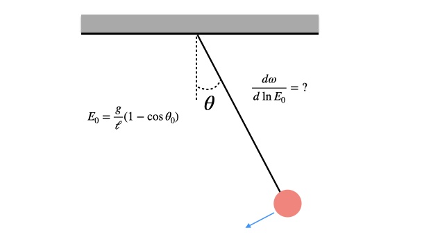
Say that we have a mass normalized (i.e., \(m=1\)) pendulum system consisting of a string of length \(\ell\). The system begins from rest with the string making an angle \(\theta_0\) with the vertical. The energy of the system is then

\begin{equation}
E_0 = \ell^2 \omega_{0}^2 (1-\cos \theta_0), \qquad (1)
\end{equation}

where \(\omega_0 = \sqrt{g/\ell}\) and \(g\) is the gravitational acceleration. The constant \(\omega_0\) is an input parameter and hence is independent of the initial energy of our system. It represents the angular frequency only in the exactly soluble case of simple harmonic motion. But for the pendulum, \(\omega_0\) is no longer the true angular frequency.

This fact represents part of the essential idea behind the renormalization group. The parameters that enter into our dynamical equation and which have particular physical interpretations for linear systems, lose that interpretation when the systems become nonlinear. In quantum field theory, there is the added fact that the nonlinearity of equations of motion is associated with divergent integral corrections to physical observables, but it is not necessary to have such divergent corrections when attempting to understand how physical quantities change with energy scale.

Period of Pendulum

To find the true angular frequency of the pendulum, we can compute the period of the pendulum from Eq.(1). This equation represents the initial energy of the system. By conservation of energy, if at some later time, the pendulum is at an angle \(\theta\) with angular velocity (\dot{\theta}\), we have the equality

\begin{equation}
\frac{1}{2}{\ell}^2\dot{\theta}^2 + \ell^2 \omega_0^2 (1-\cos\theta) = \ell^2 \omega_0^2(1-\cos\theta_0), \qquad (2)
\end{equation}

Solving this equation for \( \dot{\theta}\), we obtain

\begin{equation}
\frac{d\theta}{dt} =\omega_0{\sqrt{2(\cos\theta – \cos\theta_0)}},
\end{equation}

And solving this differential equation for the period of the pendulum which starts from rest at angle \(\theta_0\),

\begin{align}
T(\theta_0)/2 = \frac{1}{\omega_0\sqrt{2}} \int^{\theta_0}_{-\theta_0} d\theta \frac{1}{\sqrt{\cos\theta – \cos\theta_0}},
\end{align}

where we used the fact that going from \(-\theta_0 \to \theta_0\) comprises half of the period of the pendulum. With the definition \(2\pi/\omega = T\), we can rewrite this result as

\begin{equation}
\omega_0 = \frac{ \omega(\theta_0)}{\pi\sqrt{2}} \int^{\theta_0}_{-\theta_0} d\theta \frac{1}{\sqrt{\cos\theta – \cos\theta_0}} \equiv \frac{ \omega(\theta_0)}{\pi\sqrt{2}}I(\theta_0),\qquad (2)
\label{eq:int_result}
\end{equation}

where we defined the integral as \(I(\theta_0)\).

Complete Elliptic Integral

Eq.(2) gives us the true angular frequency \(\omega(\theta_0)\) as a function of the initial angle \(\theta_0\) in the system. This result is close to what we want when we pursue a “renormalization group” interpretation of the classical pendulum, but we can go a bit further to make the interpretation even more transparent. First we further reduce Eq.(2) by simplifying the integral \(I(\theta_0)\). With the identity \(\cos 0 = 1- 2\sin^2 \theta/2\), the integral becomes

\begin{equation}
I(\theta_0) = \frac{1}{\sqrt{2}} \int^{\theta_0}_{-\theta_0} d\theta \frac{1}{\sqrt{\sin^2(\theta_0/2) – \sin^2(\theta/2)}}. \end{equation}

Changing variables to \(\sin u = \sin(\theta/2)/\sin(\theta_0/2)\), we find

\begin{align} d\theta & = 2 \frac{\sin(\theta_0/2)\cos u}{\cos(\theta/2)} \, du \\ & = 2\dfrac{\sqrt{\sin^2(\theta_0/2)- \sin^2(\theta/2)}}{\sqrt{1-\sin^2(\theta/2) }} \,du, \end{align}

and so the integral is

\begin{equation}
I(\theta_0) = {\sqrt{2}}\int^{\pi/2}_{-\pi/2} du \, \frac{1}{\sqrt{1-\sin^2(\theta_0/2) \sin^2 u}} \equiv 2{\sqrt{2}}
K( \sin (\theta_0/2)),
\end{equation}

where \(K\) is the complete elliptic integral of the first kind. Returning to our expression for \(\omega_0\) in Eq.(2) we see that we have

\begin{equation}
\omega_0 = \frac{2}{\pi}\,\omega(\theta_0) K( \sin (\theta_0/2))
\end{equation}

\begin{equation}
\omega(\theta_0) = \frac{\pi}{2}\frac{\omega_0}{K(\sin(\theta_0/2))} \qquad (3),
\label{eq:omeg_act}
\end{equation}

thus giving us a reduced form for the angular frequency’s dependence on the initial angle.

Flow Equation

Now we want to reformulate the above results into a flow equation¹ which we generally represent as

\begin{equation}
\frac{d\ln \omega}{d\ln E_0}.
\end{equation}

This equation tells us how the angular frequency of the system changes with the total energy of the system. It is analogous to other more traditional renormalization group equations that tell us how physical observables like charge or mass change with energy scale.

The first step towards computing this “flow equation” is to compute the derivative of Eq.(3) with respect to the initial energy. We will do so using the chain rule. The initial energy is

\begin{equation}
E_0 = \omega_0^2(1-\cos \theta_0) = 2\omega_0^2 \sin^2(\theta_0/2).
\end{equation}
For notational simplicity, we define \(x\equiv \sin(\theta_0/2)\), so that the quantity we’re seeking is

\begin{equation}
\frac{d\omega}{dE_0} = \frac{d\omega}{dx} \frac{dx}{dE_0}. \qquad (4)
\label{eq:omeg_chng}
\end{equation}

By our definition of \(x\) we have
\begin{equation}
x = \sqrt{\frac{E_0}{2g \ell}} \quad \longrightarrow \quad \frac{dx}{dE_0} = \frac{1}{2\sqrt{2g\ell E_0}} = \frac{1}{4g\ell x}. \qquad (5)
\label{eq:xE0}
\end{equation}

From our calculation of the frequency above we have

\begin{equation}
\omega = \frac{\pi}{2} \frac{\omega_0}{K(x)},
\end{equation}

and therefore

\begin{align}
\frac{d\omega}{dx} & = – \frac{\pi}{2} \frac{\omega_0}{K(x)^2} K'(x) = – \omega \frac{d}{dx}\ln K(x) . \qquad (6)
\label{eq:omegval}
\end{align}

Next, we will make an approximation. In the small angle approximation of the pendulum, we take \(|\theta_0| \ll \pi/2\) so that the pendulum never comes close to being horizontal. For the sake of solubility, we will work in the direction of this approximation and assume \(E_0/gl\) (which is of the order of \(\theta_0^2\) in the small angle limit) is a perturbation parameter. Thus, we will compute \(K(x)\) in this limit. Employing the standard expansion of the complete integral of the first kind and taking the logarithm of the result, we obtain

\begin{align}
\ln K(x) & = \ln \left[\frac{\pi}{2}\left\{1+ \left(\frac{1}{2}\right)^2 x^2 + \left(\frac{1\cdot 3}{2\cdot 4}\right)^2 x^4+\cdots \right\}\right]\\
& = \ln(\pi/2) +\frac{1}{4}x^2 + \frac{7}{64}x^4+ \cdots.
\end{align}

The derivative is then

\begin{equation}
\frac{d}{dx}\ln K(x) = \frac{1}{2}x + \frac{7}{16}x^3 + O(x^5). \qquad (7)
\label{eq:Kd}
\end{equation}

Inserting Eq.(5), Eq.(6), and Eq.(7) into Eq.(4), we find

\begin{align}
\frac{d\omega}{dE_0} & = – \omega\left(\frac{1}{2}x + \frac{7}{16}x^3 + O(x^5)\right)\frac{1}{4g\ell x} \\
& = \,- \frac{\omega}{8g\ell} \left(1+ \frac{7}{16} \frac{E_0}{g\ell} + O(E_0^2/(gl)^2)\right). \qquad (8)
\end{align}

This is basically our final result, but we can put it in an even more illustrative form by multiplying both sides by \(E_0/\omega\). We then obtain

\begin{equation}
\boxed{\frac{d\ln \omega}{d\ln E_0} = – \frac{1}{8} \left(\frac{E_0}{g\ell}\right) – \frac{7}{128} \left(\frac{E_0}{g\ell}\right)^2 +O\left(\frac{E_0^3}{g^3 \ell^3} \right)} \qquad (9)
\label{eq:reneq}
\end{equation}

Solving Flow Equation

Eq. (9) can be interpreted as the “renormalization group equation” for the pendulum. Solving this equation (or, more specifically, solving Eq.(8)), we find

\begin{equation}
\omega(E) = \omega_0 \exp\left[-\frac{1}{8} \left(\frac{E}{g\ell}\right)-\frac{7}{256}\left(\frac{E}{g\ell}\right)^2 +{\cal O}\left(\frac{E_0^3}{g^3 \ell^3}\right)\right].
\end{equation}

which matches our intuition for the pendulum. Increasing the energy in the system leads to wider pendulum arcs, a longer period of motion, and a smaller angular frequency.

Final Remarks

OK, we’ve been mostly having fun with this example. We were able to derive an expression for how a physical quantity (i.e., the period or angular frequency) changes with the energy we add to the system. However, in most standard applications of the renormalization group changes in energy scale are more precisely changes in length scales in which we average over smaller scales to obtain a more coarse-grained system. The connection between length scale \(\ell\) and energy scale \(E\) is typically made through the particle physics convention of “natural units²” for which \(\ell \sim 1/ E\). It is mostly in this sense, that “high energy scales” are taken as proxies “smaller length scales,” so that when we find that certain parameters change according to the length scale, we can also claim that they change according to the energy scale.

Here, we have selected only this “changing energy scale” interpretation of the renormalization group to highlight that even simple (i.e., not statistical and not quantum) systems have properties that are reminiscent of those we find in more complex systems. In truth what we have shown is that nonlinear systems, whether or not they exhibit multiple length scales, have parameters that should be interpreted differently from their linear counterparts.

Footnotes

In real applications of the renormalization group, the flow equation demonstrates how coupling parameters change as we change the scale (length or energy) of the system. ↩︎
Natural units are those for which \(\hbar = 1\) and \(c=1\). Without this choice, the relationship between length scale and energy is \(\ell = \hbar c/E\). ↩︎